Working with ODEs
Physical systems can typically be modeled through differential equations, or equations including derivatives. Forces, hence Newton’s Laws, can be expressed as derivatives, as can Maxwell’s Equations, so differential equations can describe most physics problems. A differential equation describes how a system changes based on the system’s current state, in effect defining state transition. Systems of differential equations can be written in matrix/vector form:

where x is the state vector, A is the state transition matrix determined from the physical dynamics, and x dot (or dx/dt) is the change in the state with a change in time. Essentially, matrix A acts on state x to advance it a small step in time. This formulation is typically used for linear equations (where elements of A do not contain any state vector) but can be used for nonlinear equations where the elements of A may have state vectors which can lead to the complex behavior described above. This equation describes how an environment or system develops in time, starting from a particular initial condition. In mathematics, these are referred to as initial value problems since evaluating how the system will develop requires specification of a starting state.
The expression above describes a particular class of differential equations, ordinary differential equations (ODE) where the derivatives are all of one variable, usually time but occasionally space. The dot denotes dx/dt, or change in state with incremental change in time. ODEs are well studied and linear systems of ODEs have a wide range of analytic solution approaches available. Analytic solutions allow solutions to be express in terms of variables, making them more flexible for exploring the whole system behavior. Nonlinear have fewer approaches, but certain classes of systems do have analytic solutions available. For the most part though, nonlinear (and some linear) ODEs are best solved through simulation, where the solution is determined as numeric values at each time-step.
Simulation is based around finding an approximation to the differential equation, often through transformation to an algebraic equation, that is accurate to a known degree over a small change in time. Computers can then step through many small changes in time to show how the system develops. There are many algorithms available to calculate this will such as Matlab’s ODE45 or Python SciPy’s solve_ivp functions. These algorithms take an ODE and a starting point/initial condition, automatically determine optimal step size, and advance through the system to the specified ending time.
If we can apply the correct control inputs to an ODE system, we can often drive it to a desired state. As discussed last time, RL provides an approach to determine the correct inputs for nonlinear systems. To develop RLs, we will again use the gymnasium environment, but this time we will create a custom gymnasium environment based on our own ODE. Following Gymnasium documentation, we create an observation space that will cover our state space, and an action space for the control space. We initialize/reset the gymnasium to an arbitrary point within the state space (though here we must be cautious, not all desired end states are always reachable from any initial state for some systems). In the gymnasium’s step function, we take a step over a short time horizon in our ODE applying the algorithm estimated input using Python SciPy solve_ivp function. Solve_ivp calls a function which holds the particular ODE we are working with. Code is available on git. The init and reset functions are straightforward; init creates and observation space for every state in the system and reset sets a random starting point for each of those variables within the domain at a minimum distance from the origin. In the step function, note the solve_ivp line that calls the actual dynamics, solves the dynamics ODE over a short time step, passing the applied control K.
#taken from https://www.gymlibrary.dev/content/environment_creation/
#create gym for Moore-Greitzer Model
#action space: continuous +/- 10.0 float , maybe make scale to mu
#observation space: -30,30 x2 float for x,y,zand
#reward: -1*(x^2+y^2+z^2)^1/2 (try to drive to 0)#Moore-Grietzer model:
from os import path
from typing import Optional
import numpy as np
import math
import scipy
from scipy.integrate import solve_ivp
import gymnasium as gym
from gymnasium import spaces
from gymnasium.envs.classic_control import utils
from gymnasium.error import DependencyNotInstalled
import dynamics #local library containing formulas for solve_ivp
from dynamics import MGM
class MGMEnv(gym.Env):
#no render modes
def __init__(self, render_mode=None, size=30):
self.observation_space =spaces.Box(low=-size+1, high=size-1, shape=(2,), dtype=float)
self.action_space = spaces.Box(-10, 10, shape=(1,), dtype=float)
#need to update action to normal distribution
def _get_obs(self):
return self.state
def reset(self, seed: Optional[int] = None, options=None):
#need below to seed self.np_random
super().reset(seed=seed)
#start random x1, x2 origin
np.random.seed(seed)
x=np.random.uniform(-8.,8.)
while (x>-2.5 and x<2.5):
np.random.seed()
x=np.random.uniform(-8.,8.)
np.random.seed(seed)
y=np.random.uniform(-8.,8.)
while (y>-2.5 and y<2.5):
np.random.seed()
y=np.random.uniform(-8.,8.)
self.state = np.array([x,y])
observation = self._get_obs()
return observation, {}
def step(self,action):
u=action.item()
result=solve_ivp(MGM, (0, 0.05), self.state, args=[u])
x1=result.y[0,-1]
x2=result.y[1,-1]
self.state=np.array([x1.item(),x2.item()])
done=False
observation=self._get_obs()
info=x1
reward = -math.sqrt(x1.item()**2)#+x2.item()**2)
truncated = False #placeholder for future expnasion/limits if solution diverges
info = x1
return observation, reward, done, truncated, {}
Below are the dynamics of the Moore-Greitzer Mode (MGM) function. This implementation is based on solve_ivp documentation . Limits are placed to avoid solution divergence; if system hits limits reward will be low to cause algorithm to revise control approach. Creating ODE gymnasiums based on the template discussed here should be straightforward: change the observation space size to match the dimensions of the ODE system and update the dynamics equation as needed.
def MGM(t, A, K):
#non-linear approximation of surge/stall dynamics of a gas turbine engine per Moore-Greitzer model from
#"Output-Feedbak Cotnrol on Nonlinear systems using Control Contraction Metrics and Convex Optimization"
#by Machester and Slotine
#2D system, x1 is mass flow, x2 is pressure increase
x1, x2 = A
if x1>20:  x1=20.
elif x1<-20:  x1=-20.
if x2>20:  x2=20.
elif x2<-20:  x2=-20.
dx1= -x2-1.5*x1**2-0.5*x1**3
dx2=x1+K
return np.array([dx1, dx2])
For this example, we are using an ODE based on the Moore-Greitzer Model (MGM) describe gas turbine engine surge-stall dynamics¹. This equation describes coupled damped oscillations between engine mass flow and pressure. The goal of the controller is to quickly dampen oscillations to 0 by controlling pressure on the engine. MGM has “motivated substantial development of nonlinear control design” making it an interesting test case for the SAC and GP approaches. Code describing the equation can be found on Github. Also listed are three other nonlinear ODEs. The Van Der Pol oscillator is a classic nonlinear oscillating system based on dynamics of electronic systems. The Lorenz Attractor is a seemingly simple system of ODEs that can product chaotic behavior, or results highly sensitive to initial conditions such that any infinitely small different in starting point will, in an uncontrolled system, soon lead to widely divergent state. The third is a mean-field ODE system provided by Duriez/Brunton/Noack that describes development of complex interactions of stable and unstable waves as an approximation to turbulent fluid flow.
To avoid repeating analysis of the last article, we simply present results here, noting that again the GP approach produced a better controller in lower computational time than the SAC/neural network approach. The figures below show the oscillations of an uncontrolled system, under the GP controller, and under the SAC controller.


Both algorithms improve on uncontrolled dynamics. We see that while the SAC controller acts more quickly (at about 20 time steps), it is low accuracy. The GP controller takes a bit longer to act, but provides smooth behavior for both states. Also, as before, GP converged in fewer iterations than SAC.
We have seen that gymnasiums can be easily adopted to allow training RL algorithms on ODE systems, briefly discussed how powerful ODEs can be for describing and so exploring RL control of physical dynamics, and seen again the GP producing better outcome. However, we have not yet tried to optimize either algorithm, instead just setting up with, essentially, a guess at basic algorithm parameters. We will address that shortcoming now by expanding the MGM study.